Visualizing Dense and MoE Models IB Communication
TL;DR — I captured per-port, 10-millisecond resolution InfiniBand traffic during FSDP fine-tuning of Qwen-7B (dense) and Mixtral-8x7B (MoE) on Azure ND H100 v5 nodes by polling sysfs counters directly, then animated the data into frame-by-frame visualizations. At this resolution, individual FSDP collectives (AllGather, ReduceScatter) become visible as distinct ~10-30ms bursts.
The animations reveal fundamentally different communication signatures: dense models produce steady, uniform-intensity traffic thanks to FSDP’s compute-communication overlap (CV=0.20), while MoE models drive continuous but highly volatile traffic (CV=0.42) as All-to-All expert routing and FSDP collectives compete for bandwidth at varying intensities. These patterns have direct implications for network fabric design, congestion management, and cluster scheduling.
Why the Patterns Differ
The difference comes down to which NCCL collectives each architecture uses:
Dense (AllReduce-Dominated): Per-Layer Micro-Bursts
FSDP with FULL_SHARD (equivalent to ZeRO-3) actually performs three collectives per layer — not two — because it frees unsharded weights immediately after use to save memory:
- AllGather before the forward pass (fetch unsharded parameters)
- AllGather again during the backward pass (re-fetch weights, since they were freed after step 1)
- ReduceScatter after gradients are computed (sync and shard gradients)
Between these collectives, GPUs compute locally. At the per-layer level (millisecond timescale), the idealized pattern would alternate between communication and compute:
Dense timeline (without overlap):
  [AllGather] [compute] [AllGather] [grad compute] [ReduceScatter] [AllGather] ...
  ↑ IB burst  ↑ silent  ↑ IB burst  ↑ silent       ↑ IB burst      ↑ next layer

Dense timeline (with FSDP prefetch overlap — what actually happens):
  [AllGather ██████████████████████████████████████████████████████████████] ...
  [  compute ████████ ][AllGather+compute ████████ ][ReduceScatter+AG ████] ...
  ↑ IB is always busy — next layer's AllGather overlaps with current compute
In practice, modern FSDP implementations use compute-communication overlap — while the GPU computes the current layer, the IB is already prefetching (AllGather) the next layer’s parameters in the background. This overlap fills in the “silent” gaps, producing steady, uniform-intensity traffic rather than discrete bursts. The result is that dense FSDP traffic looks more like a solid block than a staircase — which is exactly what our 10ms data confirms (CV=0.20).
MoE (All-to-All + AllReduce): Continuous with Highs and Lows
MoE models add All-to-All collectives for expert routing on top of the standard FSDP collectives:
- Before each MoE layer: All-to-All to dispatch tokens to the GPUs hosting the selected experts
- After each MoE layer: All-to-All to collect expert outputs back
Unlike dense models, this means IB traffic occurs during the forward and backward passes — not just at gradient synchronization boundaries. The heatmap shows continuous traffic with varying intensity. Here’s what the highs and lows correspond to:
- Highs (bright hot bands): All-to-All expert dispatch/collect — each of Mixtral’s 32 MoE layers does two All-to-All ops, moving tokens to and from remote experts. These are layered on top of concurrent FSDP AllGather/ReduceScatter, creating peak bandwidth moments.
- Lows (dimmer but non-zero): FSDP collectives alone for non-MoE layers (attention, layer norms, embeddings). These layers behave like a dense model, but there is no extended silent gap because the next MoE layer’s All-to-All starts immediately after.
MoE timeline:
  [AllGather] [All2All ↑↑] [compute] [All2All ↑↑] [ReduceScatter] [AllGather] [All2All ↑↑] ...
              ↑ HIGH        ↑ low     ↑ HIGH                                   ↑ HIGH
The key architectural difference: without overlap, a dense model would alternate communicate → compute → communicate with silent gaps. FSDP’s prefetching fills those gaps, producing uniform traffic. In MoE, the additional All-to-All operations create bandwidth contention — FSDP collectives and expert routing compete for the same IB ports at varying intensities, producing the volatile pattern (CV=0.42) visible in the heatmap.
These All-to-All operations are also data-dependent — the traffic pattern depends on which experts the router selects for each token, making it less predictable than AllReduce’s fixed communication pattern.
Setup
| Component | Detail |
|---|---|
| VM SKU | Standard_ND96isr_H100_v5 (8× H100 80 GB, 8× 400 Gb/s NDR IB) |
| Nodes | 2-node FSDP fine-tuning |
| Models | Qwen2.5-7B (dense, 7.6B params) · Mixtral-8x7B-v0.1 (MoE, 46.7B params) |
| FSDP | FULL_SHARD, bf16, torchrun, activation checkpointing |
| Monitoring | Direct sysfs IB counter polling (/sys/class/infiniband/mlx5_ibN/ports/1/counters/), 10ms interval |
| IB Ports | 8 per node: mlx5_ib0:1 through mlx5_ib7:1 (ConnectX-7 NDR) |
Each ND H100 v5 node has 8 InfiniBand NICs, each capable of 400 Gb/s (50 GB/s) bidirectional. NCCL stripes collective operations across all 8 ports, but the pattern of that striping depends on the collective type.
The Animation
Below is a heatmap comparing all 8 IB ports (combined TX+RX bandwidth in GB/s) at 10ms resolution. The data has been trimmed to the active training window, excluding Docker startup, pip installs, and model loading.
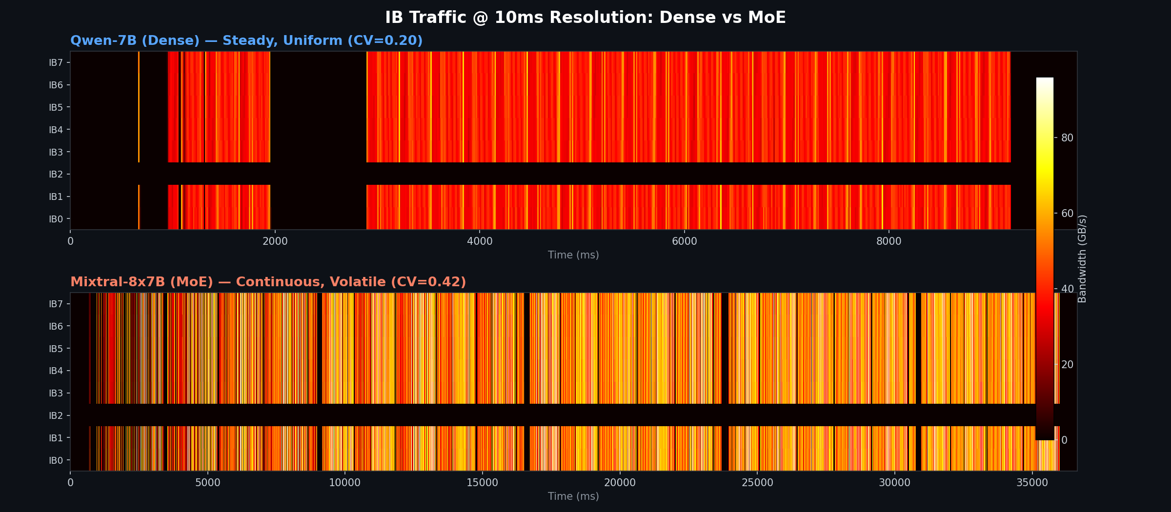
Top panel: Qwen-7B (dense) — at 10ms resolution the lifecycle of a training run becomes visible. The initial burst at ~0-40ms is NCCL topology negotiation (ring/tree setup). The short activity at ~270-650ms is the FSDP parameter unshard and the first warmup step. The second cluster (~660-1300ms) covers warmup steps 2-3. The prominent ~900ms black gap around 1300-2200ms is the torch.cuda.synchronize() + dist.barrier() between warmup and the timed benchmark — all GPUs idle while waiting for each other. Once the 20 benchmark steps begin (~2200ms onward), communication becomes nearly continuous — FSDP’s compute-communication overlap keeps the IB busy with almost no idle time.
Bottom panel: Mixtral-8x7B (MoE) — despite having more collective types (FSDP + All-to-All), the pattern shows visible black gaps between communication phases. Each 1,444ms step is long enough that gaps between forward/backward passes and step boundaries (optimizer step, gradient zeroing) become visible. The bright bands correspond to All-to-All expert dispatch/collect, while the dimmer regions are FSDP-only collectives.
For a more detailed view with per-port bar charts updating in real time, here is the rolling-window animation:
Quantitative Comparison
| Metric | Qwen-7B (Dense) | Mixtral-8x7B (MoE) |
|---|---|---|
| Sampling resolution | 10ms | 10ms |
| Training step time | 315ms | 1,444ms |
| Peak aggregate bandwidth | 463 GB/s | 659 GB/s |
| Mean bandwidth (when active) | 270 GB/s | 363 GB/s |
| Duty cycle (% of samples with >0.1 GB/s) | 74.7% | 91.6% |
| Per-port peak | ~68 GB/s | ~96 GB/s |
| Per-port mean (active) | ~39 GB/s | ~52 GB/s |
| Burstiness (coefficient of variation) | 0.20 | 0.42 |
| Active IB ports | 7 of 8 | 7 of 8 |
| Tokens/sec | 103,941 | 22,688 |
Important caveat: Mixtral-8x7B has 46.7B total parameters vs Qwen’s 7.6B, so the absolute bandwidth numbers (GB/s) are not an apples-to-apples comparison. A larger model moves more data regardless of architecture. The metrics that reflect true architectural differences are duty cycle, burstiness (CV), and communication pattern shape — these would hold even if both models were the same size.
Key observations:
- Dense traffic is steady; MoE traffic is volatile (CV=0.20 vs 0.42): When the dense model is communicating, FSDP’s compute-communication overlap produces uniform-intensity traffic (~250-350 GB/s). MoE shows higher variance because All-to-All and FSDP collectives interleave at different intensities, creating bandwidth swings.
Implications for Network Design
These different patterns stress the network fabric in fundamentally different ways:
Latency Sensitivity
| Dense | MoE | |
|---|---|---|
| Critical path | AllReduce latency between bursts | All-to-All latency during every layer |
| Tolerance | Can absorb some latency if burst throughput is high | Latency directly impacts every token in every layer |
| Impact of 10 µs extra | Minimal — hidden by compute | Compounds across 32 MoE layers per step |
MoE is more latency-sensitive because All-to-All operations happen within the forward/backward passes, not just at synchronization boundaries. Extra IB latency cannot be hidden by overlapping with compute.
Throughput Requirements
Dense models need high peak bandwidth but tolerate low average utilization. MoE needs high sustained bandwidth — the 92% duty cycle means any throughput bottleneck directly reduces training speed. In our 10ms measurements, MoE sustains ~1.3× higher average bandwidth per port (52 vs 39 GB/s when active), but the real difference is volatility — dense traffic maintains a steady state through FSDP overlap, whereas MoE forces high-intensity All-to-All spikes to constantly compete with background FSDP traffic.
Congestion and Adaptive Routing
Dense AllReduce bursts are highly synchronized — all ports fire simultaneously with predictable traffic matrices. Switch-level adaptive routing can anticipate and handle this well.
MoE All-to-All traffic is irregular and data-dependent. The router’s expert selection creates varying traffic patterns each step, making congestion harder to predict. Unlike AllReduce — which can be optimized via ring or tree algorithms that keep traffic relatively localized — All-to-All forces every GPU to exchange data with every other GPU, blasting traffic across spine switches and maximizing the chance of incast congestion on the receiver side. On multi-rail fat-tree topologies (like Azure’s ND H100 v5 fabric), this means MoE workloads are more likely to encounter transient congestion from traffic pattern collisions across jobs.
Cluster Scheduling Implications
For operators managing multi-tenant GPU clusters:
- Dense jobs can share IB bandwidth more predictably — their steady, uniform traffic profile and slightly lower duty cycle (75% vs 92%) make them easier to co-locate without triggering sudden, unpredictable network contention.
- MoE jobs are “bandwidth hogs” — near-continuous utilization means less room for other jobs to share the same IB rails without interference.
- Placing two MoE jobs on the same IB switch concurrently could cause sustained congestion, while two dense jobs would rarely collide.
Key Takeaways
| Dense (Qwen-7B) | MoE (Mixtral-8x7B) | |
|---|---|---|
| Latency sensitivity | Low — collectives occur between layers; extra latency hidden by compute overlap | High — All-to-All happens inside every MoE layer’s forward/backward pass; latency compounds across 32 layers |
| Throughput demand | High peak, tolerates idle gaps — 270 GB/s mean, 463 GB/s peak | High sustained — 363 GB/s mean, 659 GB/s peak, 92% duty cycle |
| Burstiness (CV) | 0.20 — uniform intensity when active | 0.42 — variable from interleaving All-to-All and FSDP collectives |
Related Posts
- Dense vs MoE: IB and GPU Communication Patterns
- NCCL Ring vs Tree for Multi-Node LLM Fine-Tuning
- Monitoring InfiniBand Health on Azure H100 Clusters
This is a personal blog. Opinions and recommendations are my own, not Microsoft’s.
Leave a Comment