Dense vs MoE: IB and GPU Communication Patterns
Introduction
In my previous post, I showed that Mixtral 8x7B (MoE) requires 56× more effective interconnect bandwidth than its throughput ratio would suggest, compared to a dense model of similar active size. But why? What does the communication fabric actually look like during training — and how does it differ between dense and MoE architectures?
In this post, I capture 1-second resolution InfiniBand and GPU utilization on an Azure ND H100 v5 cluster during 2-node FSDP fine-tuning of Qwen2.5-7B (dense) and Mixtral-8x7B (MoE). The data reveals strikingly different communication patterns that explain the IB sensitivity gap. Along the way, I hit thermal throttling on 2 out of 10 nodes — a real-world reminder that monitoring matters even for short benchmarks.
Test Environment
| Component | Detail |
|---|---|
| VM SKU | Standard_ND96isr_H100_v5 |
| GPUs per node | 8× NVIDIA H100 80 GB HBM3 |
| Inter-node | 8× 400 Gb/s NDR InfiniBand (ConnectX-7) |
| Nodes | 10 provisioned, 8 healthy (2 excluded — thermal issues) |
| Shared storage | Azure Managed Lustre, mounted at /lustre |
| Container | nvcr.io/nvidia/pytorch:24.12-py3 (PyTorch 2.6, CUDA 12.6, NCCL 2.23.4) |
| Monitoring | Moneo worker mode — local Prometheus per node, 1s scrape interval |
| Models | Qwen2.5-7B (7.6B params), Mixtral-8x7B-v0.1 (46.7B params) |
| FSDP | FULL_SHARD, bf16, activation checkpointing |
Thermal Throttling: The First Surprise
Before collecting any communication patterns, I ran 2-node Qwen2.5-7B benchmarks using the first two nodes from the VMSS hostfile. The result: 53,995 tokens/sec — barely half the expected ~131,000 tok/s from my earlier tests.
Diagnosis
Running Azure NHC (Node Health Checks) and GPU thermal checks across all 10 nodes revealed two problematic nodes:
Node vmssB3GCE6 (10.0.0.4):  GPU thermal throttling detected
Node vmssTSERJB:              GPU thermal throttling detected
Both nodes happened to be the first two in the hostfile — exactly the pair used for the initial benchmark. The thermal throttling was reducing GPU clock speeds, which dragged down the entire distributed job since FSDP synchronizes at every gradient step.
Resolution
I built a filtered hostfile (~/hostfile_good) containing only the 8 healthy nodes and designated a new head node:
# 8 healthy nodes
vmss72VTKQ    # new head node (10.0.0.5)
vmssH3MG2Z
vmssQF8CCJ
vmssP1A79C
vmssA72U6O
vmssFTSLKH
vmssNTAV11
vmssA8IIXN
Re-running on healthy nodes:
| Model | Nodes | GPUs | Throughput (tok/s) | Expected | Status |
|---|---|---|---|---|---|
| Qwen2.5-7B | 2 | 16 | 131,125 | ~131,018 | ✅ Match |
| Mixtral-8x7B | 2 | 16 | 22,641 | ~22,520 | ✅ Match |
Both results now match the published benchmarks. The 2.4× performance loss was entirely caused by thermal throttling on two nodes.
Lesson Learned
Always run health checks before benchmarking. At 10 nodes, 20% of the cluster had thermal issues. At scale, failing nodes are not exceptions — they’re the norm. Tools like Azure NHC and Moneo can catch these before you waste hours debugging “slow training.”
IB and GPU Patterns: Dense vs MoE
Aggregate View
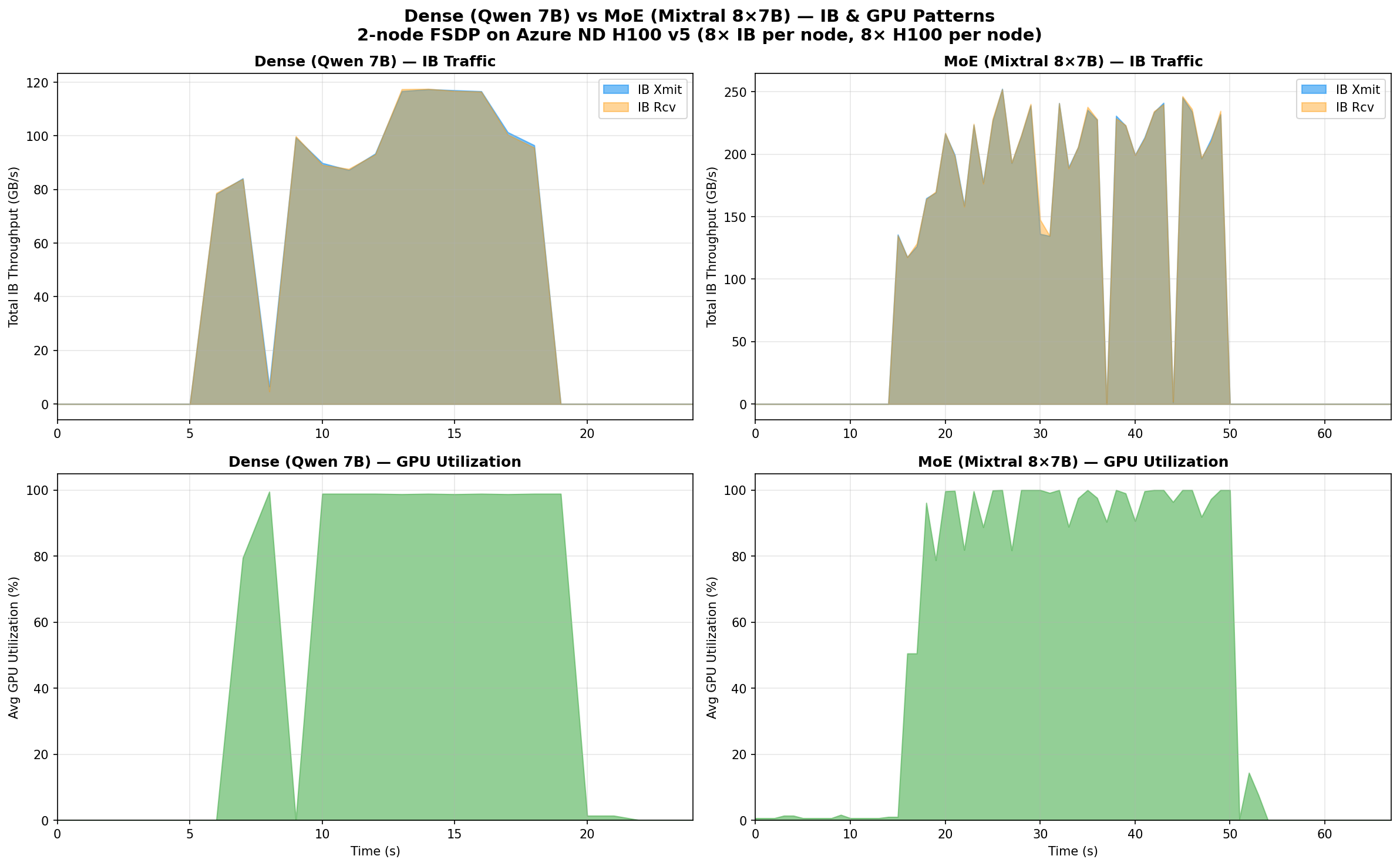
The difference is immediately visible. Let me break down the numbers:
| Metric | Dense (Qwen 7B) | MoE (Mixtral 8x7B) | Ratio |
|---|---|---|---|
| Peak total IB xmit | 117 GB/s | 252 GB/s | 2.2× |
| Peak total IB rcv | 118 GB/s | 252 GB/s | 2.1× |
| Avg IB during active | 93 GB/s | 196 GB/s | 2.1× |
| IB active window | ~12s | ~34s | 2.8× |
| Peak per-port xmit | 17.1 GB/s | 36.4 GB/s | 2.1× |
| GPU util during IB | 82% avg | 91% avg | — |
| Mean GPU util (active) | 97% | 89% | — |
| IB duty cycle | 10.7% | 11.3% | — |
Why MoE Uses 2.2× More IB Bandwidth
The bandwidth difference comes from FSDP’s FULL_SHARD strategy. During each forward+backward pass, FSDP must:
- All-gather the full parameters for each layer before computing
- Reduce-scatter the gradients after computing
The volume of data moved is proportional to the total parameter count, regardless of how many parameters are active per token.
- Qwen 7B: 7.6B parameters → ~15.2 GB in bf16 to all-gather per step
- Mixtral 8x7B: 46.7B parameters → ~93.4 GB in bf16 to all-gather per step
That’s a 6.1× ratio in raw parameter count. The measured 2.2× IB ratio is lower because:
- FSDP pipelines communication with computation (overlapping all-gather with forward pass)
- Mixtral’s longer computation time (MoE layers with expert routing) gives more time for communication to hide behind compute
- The training step is longer for Mixtral (~1,447ms vs ~500ms), so the same data moves over a wider window
Computation vs Communication Overlap
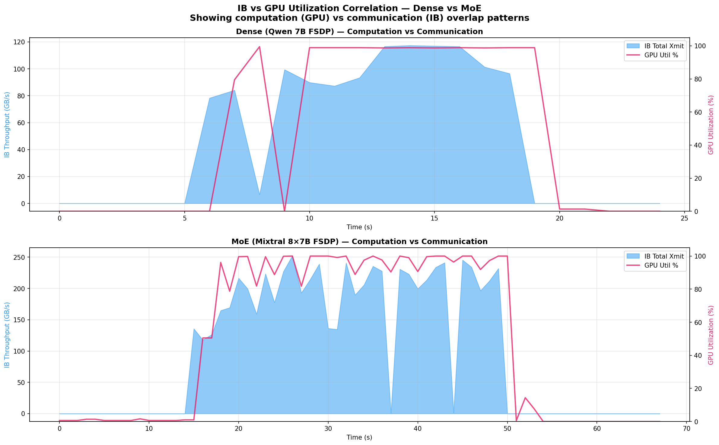
The overlay view reveals the key architectural difference:
Dense (Qwen 7B): GPU utilization and IB traffic are tightly coupled. During the active training window, GPUs hit 97% average utilization while IB bursts carry 86 GB/s. The model is compute-dominated — the 7.6B parameters create moderate communication that overlaps efficiently with computation.
MoE (Mixtral 8x7B): The pattern is more complex. IB traffic is higher (196 GB/s average) and more sustained (34s vs 12s active window), while GPU utilization averages only 89% — 8 percentage points lower than the dense model. This gap reveals communication pressure: the 46.7B total parameters generate so much FSDP traffic that computation occasionally stalls waiting for all-gather to complete.
The overlap analysis confirms this:
| Overlap | Dense (Qwen 7B) | MoE (Mixtral 8x7B) |
|---|---|---|
| Both IB + GPU active | 11 samples | 33 samples |
| IB only (GPU idle) | 2 samples | 1 sample |
| GPU only (no IB) | 1 sample | 4 samples |
| GPU util during IB bursts | 82% | 91% |
Per-Port IB Breakdown
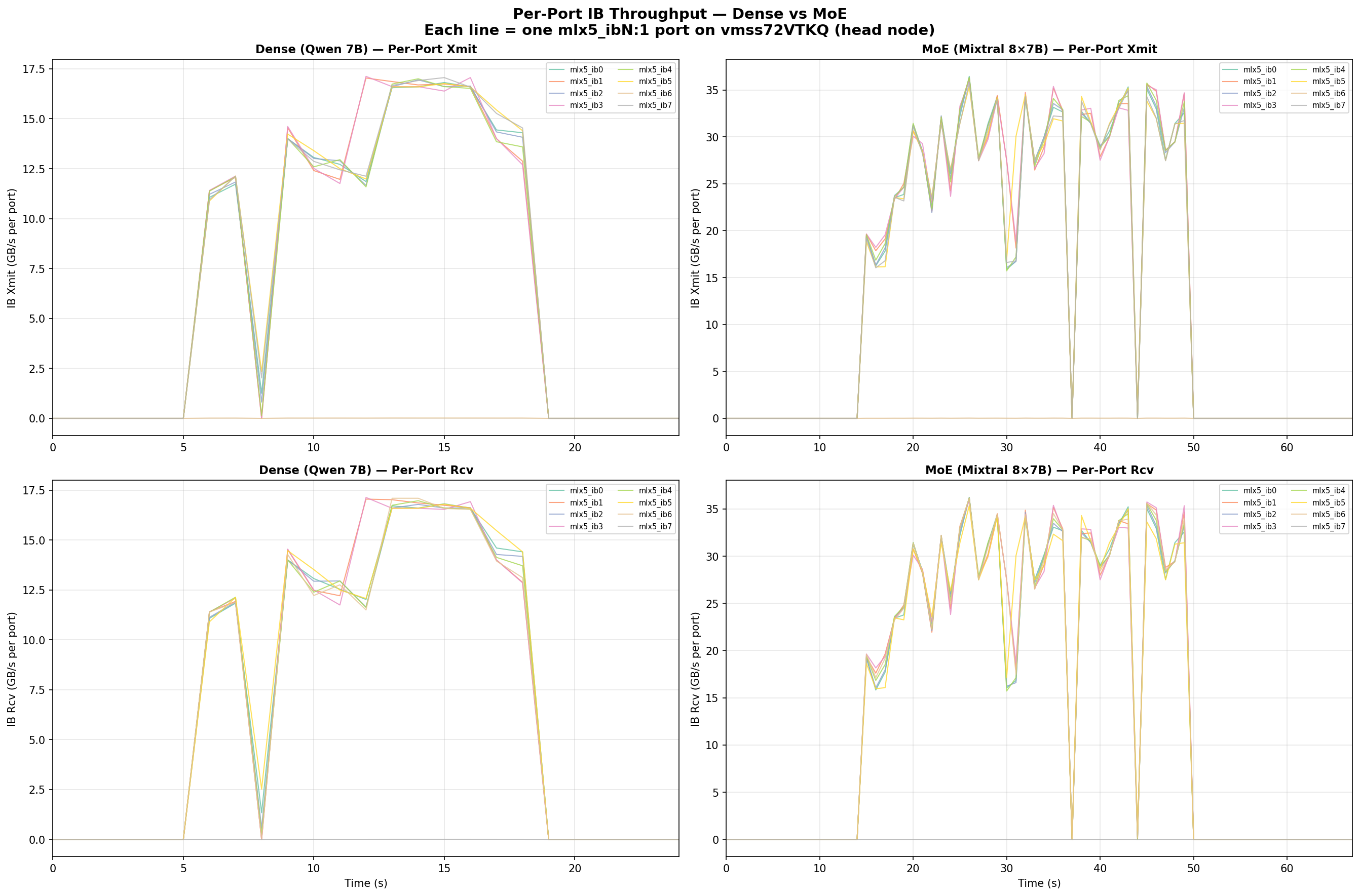
Each Azure ND H100 v5 node has 8 InfiniBand HCAs (mlx5_ib0 through mlx5_ib7). The per-port view shows:
- Ports 0–5, 7 carry traffic evenly — 16–17 GB/s peak each for Qwen, 35–36 GB/s for Mixtral
- Port 6 (
mlx5_ib6) consistently shows near-zero xmit but normal rcv — this port serves a different function in the Azure IB topology (asymmetric routing) - NCCL distributes traffic across all active ports efficiently — no single port is a bottleneck
The per-port peaks represent 42–45% of the 400 Gb/s (50 GB/s) theoretical maximum per NDR port, which is typical for a 2-node all-reduce workload where the ring algorithm doesn’t fully saturate every link.
Why This Matters for Architecture Selection
The data quantifies a fundamental trade-off in MoE design:
MoE models are more communication-hungry than their active parameter count suggests. Mixtral-8x7B has only 12.9B active parameters per token (comparable to a 13B dense model), but its FSDP communication volume scales with the 46.7B total parameters. This makes the interconnect 3.6× more critical per useful FLOP compared to a dense model of similar inference cost.
This explains the results from my previous post:
| Model | IB/ETH Speedup | Communication Sensitivity |
|---|---|---|
| Qwen 7B (dense) | 26–28× | Moderate |
| Qwen 72B (dense) | 45× | High |
| Mixtral 8x7B (MoE) | 56–57× | Very High |
Mixtral’s 56× IB/ETH gap isn’t just because it’s a bigger model — it’s because the MoE architecture has a structurally worse compute-to-communication ratio. Every training step must all-gather 46.7B parameters but only uses 12.9B for computation.
Reproducing These Results
Prerequisites
- Azure VMSS with
Standard_ND96isr_H100_v5nodes (minimum 2 nodes) - Azure Managed Lustre mounted at
/lustre - Moneo deployed in worker mode for monitoring
- Models downloaded to
/lustre/models/
Scripts
All scripts are available in the replication directory:
Dense (Qwen 7B) benchmark:
finetune_bench.py— FSDP training loop with synthetic datalaunch_node.sh— Docker container launcher per noderun_multinode.sh— Orchestrator (reads~/hostfile_good, manages SSH)
MoE (Mixtral 8x7B) benchmark:
finetune_bench_moe.py— MoE-specific FSDP withtransformer_auto_wrap_policytargetingMixtralDecoderLayerlaunch_node_moe.sh— Docker launcher withacceleratedependencyrun_multinode_moe.sh— MoE orchestrator
Visualization:
plot_patterns_v2.py— Generates all three comparison figures from Prometheus JSON exportsanalyze_patterns.py— Detailed numerical analysis of IB/GPU patterns
Running the Benchmarks
# SSH to the head node
ssh -i azureuser_id_rsa -p 50000 azureuser@<public_ip>

# Deploy scripts to Lustre (accessible from all nodes)
sudo mkdir -p /lustre/scripts
sudo cp finetune_bench.py launch_node.sh run_multinode.sh /lustre/scripts/
sudo cp finetune_bench_moe.py launch_node_moe.sh run_multinode_moe.sh /lustre/scripts/

# Run Dense benchmark (2 nodes, InfiniBand)
bash /lustre/scripts/run_multinode.sh 2 0 /lustre/models/Qwen2.5-7B 2048 2 20

# Run MoE benchmark (2 nodes, InfiniBand)
bash /lustre/scripts/run_multinode_moe.sh 2 0 /lustre/models/Mixtral-8x7B-v0.1 2048 1 20
Collecting Metrics
Moneo’s Prometheus on each node stores data locally. Export via the API:
# Query from the head node's local Prometheus
curl -s 'http://localhost:9090/api/v1/query_range' \
  --data-urlencode 'query=ib_port_xmit_data' \
  --data-urlencode 'start=2026-03-15T05:04:30Z' \
  --data-urlencode 'end=2026-03-15T05:06:30Z' \
  --data-urlencode 'step=1s' > qwen_ib_xmit.json

# GPU utilization
curl -s 'http://localhost:9090/api/v1/query_range' \
  --data-urlencode 'query=dcgm_gpu_utilization' \
  --data-urlencode 'start=2026-03-15T05:04:30Z' \
  --data-urlencode 'end=2026-03-15T05:06:30Z' \
  --data-urlencode 'step=1s' > qwen_gpu_util.json
Note: Each node’s Prometheus only scrapes its own exporters. To get cluster-wide data, you’d need to query each node separately or set up a centralized Prometheus.
Key Takeaways
-
MoE models generate 2.2× more IB traffic than comparably-sized dense models (measured peak: 252 vs 117 GB/s across 8 IB ports) because FSDP all-gathers are proportional to total parameters (46.7B), not active parameters (12.9B).
-
Dense models achieve higher GPU utilization (97% vs 89% average) because their lower communication volume overlaps more efficiently with computation.
-
Thermal throttling on even 2 out of 10 nodes caused a 2.4× throughput drop — distributed training synchronizes every step, so the slowest node dictates cluster performance.
-
Moneo’s net_exporter reports deltas, not cumulative counters — query raw gauge values, not
rate(). -
NCCL distributes traffic evenly across 7 of 8 IB ports — port 6 (
mlx5_ib6) has asymmetric behavior in the Azure IB topology.
Related Posts
- InfiniBand vs Ethernet for Multi-Node LLM Fine-Tuning — the throughput benchmarks that motivated this analysis
- Monitoring IB Counters with Prometheus and Grafana — the monitoring pipeline used to collect this data
- AMLFS with GPU VMSS — setting up Azure Managed Lustre for shared model storage
This is a personal blog. Opinions and recommendations are my own, not Microsoft’s.
Leave a Comment