Experiments on NCCL Ring vs Tree
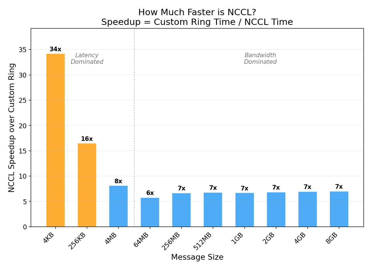
We implement a ring allreduce algorithm from scratch in Python, run it on 16 NVIDIA H100 GPUs across 2 nodes with InfiniBand, and benchmark it against NCCL’s optimized allreduce. NCCL wins by 7x on large messages and 34x on small messages — here’s exactly why.
What is AllReduce?
AllReduce is the most important collective communication operation in distributed deep learning. It takes a tensor from every GPU, reduces them (typically sum), and distributes the result back to all GPUs:
Before AllReduce (sum):
  GPU 0: [1, 2, 3]
  GPU 1: [4, 5, 6]
  GPU 2: [7, 8, 9]
  GPU 3: [10, 11, 12]

After AllReduce (sum):
  GPU 0: [22, 26, 30]    ← same result on every GPU
  GPU 1: [22, 26, 30]
  GPU 2: [22, 26, 30]
  GPU 3: [22, 26, 30]
In DDP (DistributedDataParallel) training, allreduce is called after every backward pass to average gradients across all GPUs, keeping model replicas in sync.
Ring AllReduce: The Algorithm
The naive approach — gather everything to one GPU, sum it, broadcast back — creates a bottleneck at the root. Ring allreduce solves this by arranging GPUs in a logical ring and splitting the work across all participants.
Phase 1: Reduce-Scatter
Each GPU splits its data into N chunks (one per GPU). Over N-1 steps, chunks rotate around the ring, accumulating partial sums at each hop. After this phase, each GPU holds the complete sum of exactly one chunk.
4 GPUs, data split into 4 chunks [A, B, C, D]

Initial state:
  GPU 0: [A0, B0, C0, D0]     (subscript = which GPU's data)
  GPU 1: [A1, B1, C1, D1]
  GPU 2: [A2, B2, C2, D2]
  GPU 3: [A3, B3, C3, D3]

Step 1: Each GPU sends one chunk right, receives from left, accumulates:
  GPU 0: [_, _, _, D0+D3]     ← received D3 from GPU 3, added to D0
  GPU 1: [A0+A1, _, _, _]     ← received A0 from GPU 0, added to A1
  GPU 2: [_, B1+B2, _, _]     ← received B1 from GPU 1, added to B2
  GPU 3: [_, _, C2+C3, _]     ← received C2 from GPU 2, added to C3

Step 2: Rotate again:
  GPU 0: [_, _, C2+C3+C0, _]
  GPU 1: [_, D0+D3+D1, _, _]
  GPU 2: [A0+A1+A2, _, _, _]
  GPU 3: [_, _, _, B1+B2+B3]

Step 3: Final rotation:
  GPU 0: [_, B1+B2+B3+B0, _, _]  ← GPU 0 owns complete sum of chunk B
  GPU 1: [_, _, C2+C3+C0+C1, _]  ← GPU 1 owns complete sum of chunk C
  GPU 2: [_, _, _, D0+D3+D1+D2]  ← GPU 2 owns complete sum of chunk D
  GPU 3: [A0+A1+A2+A3, _, _, _]  ← GPU 3 owns complete sum of chunk A
Phase 2: AllGather
Now each GPU has one completed chunk. Over another N-1 steps, the completed chunks rotate around the ring until every GPU has all chunks:
Step 1: Each GPU sends its completed chunk right:
  GPU 0: [A_sum, B_sum, _, _]
  GPU 1: [_, B_sum, C_sum, _]
  ...

Step 2–3: Continue rotating until all GPUs have all chunks.

Final state:
  GPU 0: [A_sum, B_sum, C_sum, D_sum]  ← complete result
  GPU 1: [A_sum, B_sum, C_sum, D_sum]
  GPU 2: [A_sum, B_sum, C_sum, D_sum]
  GPU 3: [A_sum, B_sum, C_sum, D_sum]
Why Ring is Bandwidth-Optimal
Each GPU sends and receives exactly 2 × (N-1)/N × data_size bytes total. With N=16, that’s 2 × 15/16 = 1.875× the data. This is independent of the number of GPUs — adding more GPUs doesn’t increase per-GPU bandwidth cost. The bottleneck is only the per-link bandwidth, not the GPU count.
Tree AllReduce: The Alternative
Tree AllReduce uses a binary tree topology instead of a ring:
Phase 1 — Reduce (bottom-up):

        GPU 0 (root)
       /            \
    GPU 1          GPU 2
   /    \         /    \
 GPU 3  GPU 4  GPU 5  GPU 6

  Leaves send to parents.
  Parents sum and forward up.
  Root has the final sum.

Phase 2 — Broadcast (top-down):

  Root sends result down to all leaves.
Latency: 2 × log₂(N) steps — much fewer than Ring’s 2 × (N-1) steps. With 16 GPUs: Tree = 8 steps, Ring = 30 steps.
Bandwidth: The root is a bottleneck — it must process all data. Less efficient than Ring for large messages.
When to Use Each
| Ring | Tree | |
|---|---|---|
| Best for | Large messages (>256KB) | Small messages (<256KB) |
| Latency | O(N) steps | O(log N) steps |
| Bandwidth | Optimal | Root bottleneck |
| NCCL default | Used for large collectives | Used for small collectives |
NCCL automatically selects the algorithm based on message size. For the gradient allreduce in training (typically hundreds of MB), it almost always picks Ring.
Our Experiment: Custom Ring vs NCCL
We implemented Ring AllReduce from scratch in Python using PyTorch’s dist.batch_isend_irecv for point-to-point communication, then benchmarked it against NCCL’s optimized dist.all_reduce on a real multi-node H100 cluster.
Setup
- Cluster: 2 nodes, Azure ND H100 v5 (Standard_ND96isr_H100_v5)
- GPUs: 16 × NVIDIA H100 80GB HBM3
- Interconnect: NVLink intra-node, 8× 400 Gbps InfiniBand inter-node
- Container:
nvcr.io/nvidia/pytorch:24.12-py3(NCCL 2.28.9)
The Implementation
The core of our custom Ring AllReduce:
def ring_allreduce(tensor, group=None):
    world_size = dist.get_world_size(group)
    rank = dist.get_rank(group)
    chunks = list(tensor.view(-1).chunk(world_size))
    left = (rank - 1) % world_size
    right = (rank + 1) % world_size
    recv_buf = torch.zeros_like(chunks[0])

    # Phase 1: Reduce-Scatter (N-1 steps)
    for step in range(world_size - 1):
        send_idx = (rank - step) % world_size
        recv_idx = (rank - step - 1) % world_size
        ops = [
            dist.P2POp(dist.isend, chunks[send_idx], right),
            dist.P2POp(dist.irecv, recv_buf, left),
        ]
        reqs = dist.batch_isend_irecv(ops)
        for req in reqs:
            req.wait()
        chunks[recv_idx].add_(recv_buf)

    # Phase 2: AllGather (N-1 steps)
    for step in range(world_size - 1):
        send_idx = (rank - step + 1) % world_size
        recv_idx = (rank - step) % world_size
        ops = [
            dist.P2POp(dist.isend, chunks[send_idx], right),
            dist.P2POp(dist.irecv, recv_buf, left),
        ]
        reqs = dist.batch_isend_irecv(ops)
        for req in reqs:
            req.wait()
        chunks[recv_idx].copy_(recv_buf)

    tensor.view(-1).copy_(torch.cat(chunks))
Correctness Verification
Both implementations produce identical results, verified on all 16 GPUs:
Correctness verification:
  Custom Ring AllReduce: PASS ✓
  NCCL AllReduce:        PASS ✓
  Ring == NCCL:          PASS ✓
Results
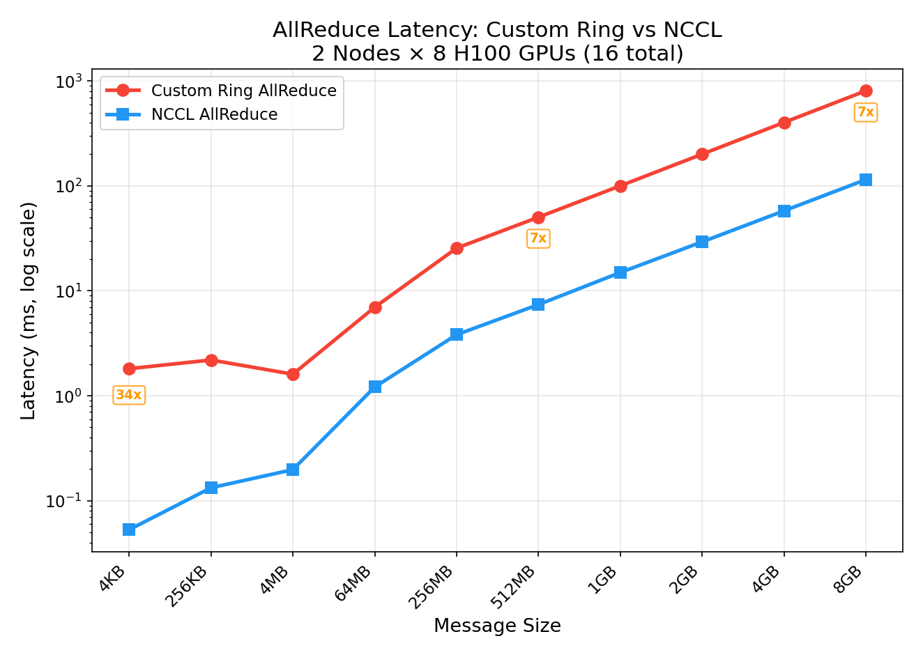
| Size | Custom Ring | NCCL | NCCL Speedup |
|---|---|---|---|
| 4 KB | 1.81 ms | 0.05 ms | 34x |
| 256 KB | 2.19 ms | 0.13 ms | 17x |
| 4 MB | 1.61 ms | 0.20 ms | 8x |
| 64 MB | 6.99 ms (18 GB/s) | 1.21 ms (104 GB/s) | 6x |
| 512 MB | 50.3 ms (20 GB/s) | 7.40 ms (136 GB/s) | 7x |
| 8 GB | 806 ms (20 GB/s) | 115 ms (140 GB/s) | 7x |
Why NCCL is 7x Faster (Large Messages)
Our custom Ring and NCCL use the same algorithm — both are ring allreduce, both are bandwidth-optimal in theory. The 7x gap comes entirely from implementation:
-
Kernel fusion: NCCL fuses send + reduce + recv into a single GPU kernel per step. Our implementation issues separate
isend,irecv,wait, andadd_calls — 4 kernel launches per step instead of 1. -
Pipelining: NCCL splits each chunk into sub-chunks and pipelines them — step N+1’s send begins before step N’s recv completes. Our code strictly waits for each step to finish before starting the next.
-
Channel parallelism: NCCL runs multiple rings in parallel (8-32 channels), each carrying a different slice of data. Our code uses a single ring.
-
GPUDirect RDMA: NCCL transfers data directly between GPU memory over InfiniBand via GPUDirect, bypassing CPU entirely. Our
batch_isend_irecvgoes through the PyTorch dispatcher and NCCL’s p2p API, adding CPU overhead per step. -
Protocol selection: For large messages, NCCL uses the “Simple” protocol with large GPU-side buffers. For small messages, it uses “LL” (Low-Latency) with inline data. Our code uses the same p2p path regardless of size.
Why NCCL is 34x Faster (Small Messages)
For small messages (4 KB), our custom ring pays 15 round-trip latencies (N-1 = 15 steps, each with a wait() sync). Each step has ~120μs of overhead even though the data itself is tiny. NCCL’s tree algorithm completes the same operation in one fused kernel launch with only 4 steps (log₂(16) = 4).
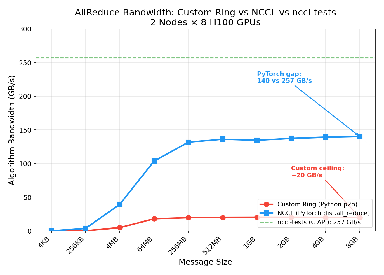
Comparison with nccl-tests
We also compared our PyTorch-based NCCL benchmark against nccl-tests (the official NCCL C benchmarking tool) run with optimized parameters:
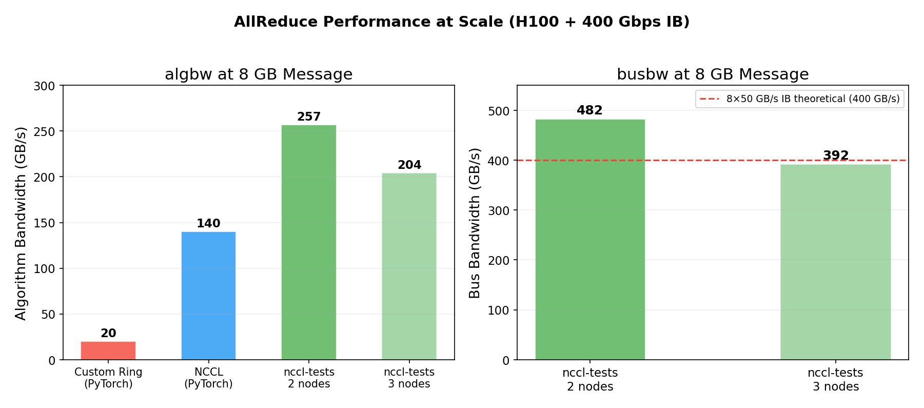
| Benchmark | algbw (8GB) | busbw (8GB) |
|---|---|---|
| Custom Ring (Python p2p) | 20 GB/s | — |
| NCCL via PyTorch | 140 GB/s | — |
| nccl-tests (2 nodes) | 257 GB/s | 482 GB/s |
| nccl-tests (3 nodes) | 204 GB/s | 392 GB/s |
The gap between PyTorch (140 GB/s) and nccl-tests (257 GB/s) comes from:
- NCCL tuning: nccl-tests was run with
NCCL_MIN_NCHANNELS=32(32 parallel rings) andNCCL_IB_QPS_PER_CONNECTION=4— our PyTorch benchmark used defaults - Direct C API: nccl-tests calls NCCL’s C API directly, avoiding PyTorch dispatch overhead
- Minimal benchmark overhead: nccl-tests has zero Python, zero tensor metadata, zero GIL
The 482 GB/s busbw on 2 nodes means each of the 8 InfiniBand ports is running at ~49 GB/s — 98% of the 50 GB/s line rate. This is essentially perfect hardware utilization.
The 3-node run drops to 392 GB/s busbw because more ring hops cross the slower IB links instead of fast NVLink. With 2 nodes, only 2 out of 16 ring hops cross IB (12.5%); with 3 nodes, 6 out of 24 cross IB (25%).
Key Takeaways
-
The algorithm is correct but the implementation matters enormously. Our Ring AllReduce produces identical results to NCCL, but is 7x slower at large messages due to Python overhead, lack of pipelining, and single-channel operation.
-
NCCL’s main advantage is engineering, not algorithms. Both use ring allreduce for large messages. NCCL wins through kernel fusion, multi-channel parallelism, GPUDirect RDMA, and protocol adaptation.
-
Small messages are latency-bound. At 4 KB, our ring takes 1.8ms (15 sequential steps × ~120μs each). NCCL’s tree algorithm takes 0.05ms (4 steps in one fused kernel). For gradient allreduce in training this doesn’t matter (gradients are hundreds of MB), but it matters for frequent small collectives.
-
NCCL tuning parameters have a large impact. Default NCCL achieves 140 GB/s; with
NCCL_MIN_NCHANNELS=32andNCCL_IB_QPS_PER_CONNECTION=4, it reaches 257 GB/s — an 83% improvement from tuning alone. -
H100 IB bandwidth is nearly fully saturated at scale. The 482 GB/s busbw on 2 nodes shows 98% IB line-rate utilization. This is what a healthy Azure ND H100 v5 cluster looks like.
Reproduce This
The benchmark script is available at allreduce_benchmark.py. To run on 2 nodes:
# Worker node (background):
torchrun --nnodes=2 --nproc_per_node=8 --node_rank=1 \
  --master_addr=<HEAD_IP> --master_port=29500 allreduce_benchmark.py

# Head node (foreground):
torchrun --nnodes=2 --nproc_per_node=8 --node_rank=0 \
  --master_addr=<HEAD_IP> --master_port=29500 allreduce_benchmark.py
Experiments run on Azure ND H100 v5 (Standard_ND96isr_H100_v5) with NCCL 2.28.9 and 400 Gbps InfiniBand. All measurements are from actual GPU runs, not estimates.
This is a personal blog. Opinions and recommendations are my own, not Microsoft’s.
Leave a Comment